Dynamic Factor Models: Stock and Option Volume

A previous post analyzed the cycles in stock and options volume. This post seeks to expand on that topic using a different technique. While that previous post examined individual companies, this post will look at the markets as a whole. Using a dynamic factor model to extract a common factor between stock and option trading volume I find that the common factor is mostly driven by stocks. In addition the impulse response functions indicate periodic dampening.

A dynamic factor model takes two or more series of data and considers whether there are some common, unobserved forces (the factors) that influences those variables. For instance, in this stock and options exercise that common factor might be market enthusiasm. Since we don't observe the factor we can't actually give it a name. Dynamic factor models generate results that tell us how correlated the factor is with each variable and how much each variable contributed to determining the factor.

I will use the NYSE trade volume data, and the VBOE options data, which are daily volume statistics from November 1, 2006 on. I find that the factor loadings (correlation of the variables with the underlying factor) are 0.42 and 0.30 for stocks and options, respectively. The coefficients of determination (the degree to which each variable contributed to the factor) are 0.99 for stocks and 0.19 for options. These numbers tell us that this unobserved factor can explain about a third of the growth rates for trade volume in stock and options markets. Further, stock market trade volume is the primary driver of the common force that drives these markets. Finally, we look to the impulse response function: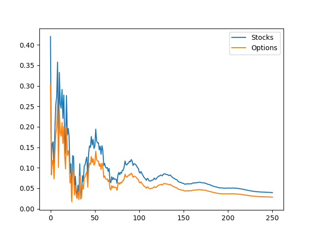

An impulse response function is a graph of what happens to the variables of interest if there is a one time shock (increase or decrease of the variable). That is, suppose the factor increases by 1% today, and impulse response function test us the impact of that 1 percent growth have on the subsequent days of trading. A critical component of this is that there are no additional shocks on the subsequent days. For our data, you can see that the first period has an increase equal to the factor loading, if the factor goes up by 1, stock volume goes up by 0.42 etc.

The surprising part of this graph is the periodic dampening effect. This leads me to believe that the factor is measuring some sort of herd behavior or enthusiasm cycle (Keynes' "animal spirits" comes to mind). When there is a spike in trading, participants back off to assess the situation, as that happens, the market starts to look more attractive so they pile back in, leading to another (smaller) spike and so on.